chainsawriot
Home | About | ArchiveR performance tuning #2
Previously on this blog: #1
I would like first to develop the data-driven idea a little bit more.
Performance profiling
How you set up the test always influences the outcome of the test. For example, if the test data is just one NULL, you probably won’t see much performance variation. This is how the test dataset is generated:
.create <- function(candidate = c(LETTERS, letters, c("\"", "<",">", "&", "'", " ")), min = 1, max = 400) {
    paste(sample(x = candidate, size = sample(seq(min, max), 1), replace = TRUE), collapse = "")
}
A brief analysis found that around 97% of the generated data contain those special characters; with a mean of 200 characters. I don’t have a reliable estimate, but it is probably not realistic that 97% of the data that pass through readODS::write_ods would need escaping. htmltools::htmlEscape() tests whether the input needs to be escaped first. In a situation where escaping is rare, this approach might have advantage.
However, it is difficult to say for sure what test dataset is realistic. It is just like real life: It is difficult to say any given test (e.g. an exam) can certainly reflect the realistic performance of the test takers. Right? Crammers.
A better approach, instead, is to create a performance profile: adjusting the test data by different parameters and see how the performance changes. As a simple model for our example, there are two parameters: percentage of data needs to be escaped (p_escape) and number of characters (nchars).
.create <- function(p_escape, nchars) {
    if (rbinom(1, 1, p_escape) == 1) {
        return(paste(c(c("\"", "<",">", "&", "'", " "), sample(x = c(LETTERS, letters,c("\"", "<",">", "&", "'", " ")), size = nchars, replace = TRUE)), collapse = ""))
    }
    paste(sample(x = c(LETTERS, letters), size = nchars, replace = TRUE), collapse = "")
}
For example, in the situation of p_escape = 0 and nchars = 10, htmltools::htmlEscape() is still the slowest. The performance of the tuned implementation is 3x its performance.
data <- replicate(300000, .create(p_escape = 0, nchars = 10))
bench::mark(output1 <- .escape_xml2(data),
	        output2 <- .escape_xml(data),
            output3 <- .html_escape(data),
            min_time = 5)
It’s better to test various conditions to have a more comprehensive look of the performance profile.
conditions <- expand.grid(p_escape = c(0, 0.01, 0.1, 0.5, 1), nchars = c(1, 10, 100, 200, 1000))

.bench <- function(p_escape, nchars) {
    message(p_escape, "/", nchars)
    data <- replicate(10000, .create(p_escape = p_escape, nchars = nchars)) ## lower
    bench::mark(output <- .escape_xml2(data),
                output2 <- .escape_xml(data),
                output3 <- .html_escape(data),
                min_time = 2) ## also lower
}
require(dplyr)
require(ggplot2)
res <- purrr::map2(conditions$p_escape, conditions$nchars, .bench)
cbind(conditions, purrr::map_dfr(res, ~as.data.frame(t(.[,"median"])))) %>%
    rename("escape_xml2" = "V1", "escape_xml" = "V2", "html_escape" = "V3") %>%
    remove_rownames() %>%
    pivot_longer(escape_xml2:html_escape, names_to = "fx", values_to = "time") %>%
	mutate(fx = forcats::fct_relevel(fx, "escape_xml2")) %>%
    ggplot(aes(x = p_escape, y = time, col = `fx`)) + geom_line() + geom_point() +
    facet_grid(rows = vars(nchars), scales = "free_y") + theme_minimal() -> img
ggsave("tuning_vis1.png", img)
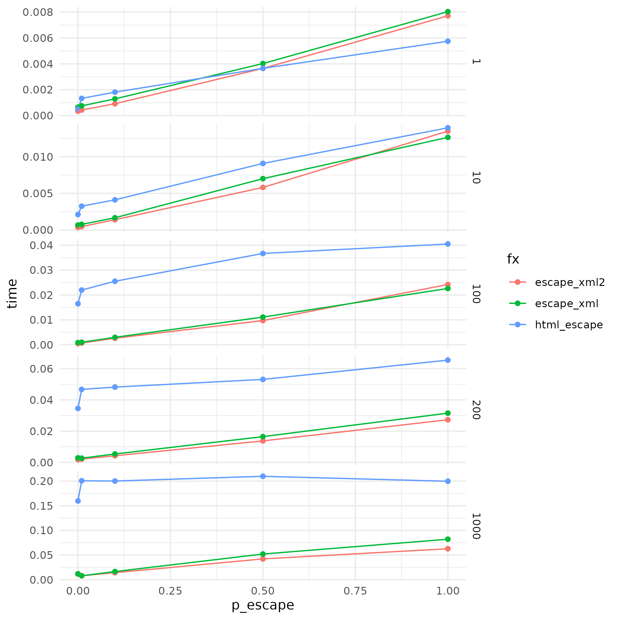
With this performance profile, we know that p_escape in general increases the processing time for all functions. But htmltools::htmlEscape() has no performance improvement even when p_escape is low. Also, the performance increase over htmltools::htmlEscape() is more visible when nchars is bigger.
Of course, one can still argue the conditions can still be artificial and the same argument of “How you set up the test always influences the outcome of the test” still exists. But this is much better than just one test.
Go compiled
To further optimize, the way is to rewrite the function in a compiled language. Usually C++.
This is modified from an implementation of XML escaping on Stackoverflow in C++. Probably not the most efficient algorithm, but I can somehow understand it.
#include <string>
// [[Rcpp::export]]
std::string encode(std::string& data) {
std::string buffer;
buffer.reserve(data.size());
for(size_t pos = 0; pos != data.size(); ++pos) {
switch(data[pos]) {
case '&': buffer.append("&"); break;
case '\"': buffer.append("""); break;
case '\'': buffer.append("'"); break;
case '<': buffer.append("<"); break;
case '>': buffer.append(">"); break;
default: buffer.append(&data[pos], 1); break;
}
}
return buffer;
}
Wrapping this with Rcpp is kind of straightforward. But that’s not vectorized and not NA conscious.
require(Rcpp)
## save the above C++ as `encode.cpp`
Rcpp::sourceCpp("encode.cpp")
x <- "You & Me, I love \"you\" > than you do."
encode(x)
encode(c(x, x)) ## error
To make the function vectorize and NA conscious:
#include <string>
#include <Rcpp.h>
using namespace Rcpp;
std::string encode(std::string& data) {
std::string buffer;
buffer.reserve(data.size());
for(size_t pos = 0; pos != data.size(); ++pos) {
switch(data[pos]) {
case '&': buffer.append("&"); break;
case '\"': buffer.append("""); break;
case '\'': buffer.append("'"); break;
case '<': buffer.append("<"); break;
case '>': buffer.append(">"); break;
default: buffer.append(&data[pos], 1); break;
}
}
return buffer;
}
// [[Rcpp::export]]
CharacterVector vencode(CharacterVector& data) {
int n = data.length();
CharacterVector output(n);
for (int i = 0; i < n; ++i) {
if(CharacterVector::is_na(data[i])) {
output[i] = NA_STRING;
} else {
std::string line = as<std::string>(data[i]);
output[i] = encode(line);
}
}
return output;
}
And benchmark it.
.bench2 <- function(p_escape, nchars) {
    message(p_escape, "/", nchars)
    data <- replicate(10000, .create(p_escape = p_escape, nchars = nchars))
    bench::mark(output3 <- .escape_xml2(data),
                output2 <- vencode(data),
                min_time = 2)
}
res <- purrr::map2(conditions$p_escape, conditions$nchars, .bench2)
cbind(conditions, purrr::map_dfr(res, ~as.data.frame(t(.[,"median"])))) %>%
    rename("escape_xml2" = "V1", "vencode" = "V2") %>%
    remove_rownames() %>%
    pivot_longer(escape_xml2:vencode, names_to = "fx", values_to = "time") %>%
    ggplot(aes(x = p_escape, y = time, col = `fx`)) + geom_line() + geom_point() +
    facet_grid(rows = vars(nchars), scales = "free_y") + theme_minimal() -> img
ggsave("tuning_vis2.png", img)
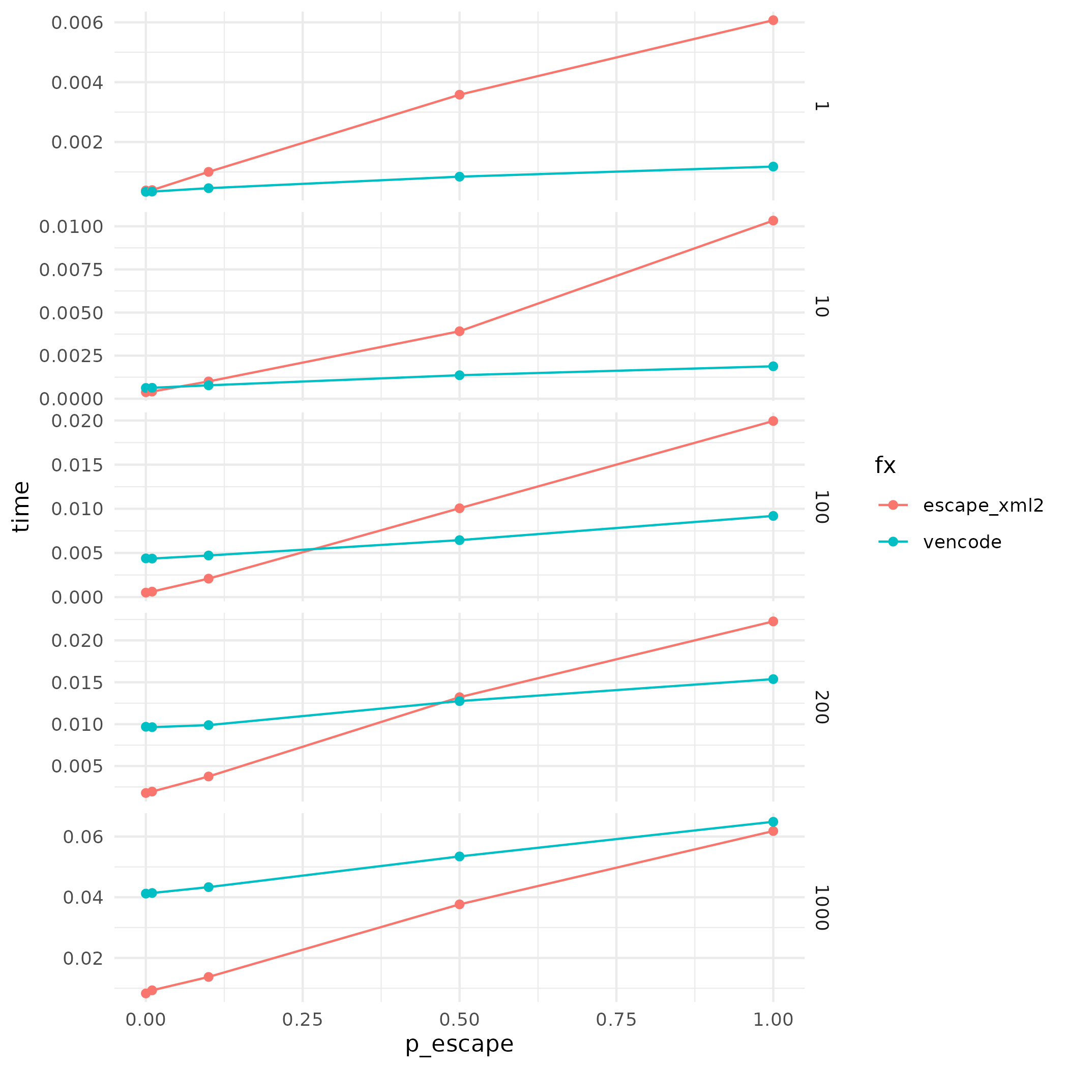
Using the same performance profiling approach, the C++ rewrite has performance advantage when p_escape is large. As a matter of fact, the performance of the C++ version does not appear to be affected by p_escape. The C++ rewrite is not faster when nchars is 1000. As most of the data passing through the XML escape is shorter than 1000 characters, writing the function in C++ still offers performance improvement.
The problem, however, is that readODS uses cpp11 rather than Rcpp. Rewriting the C++ code for cpp11 is okay.
#include <string>
#include <cpp11.hpp>
std::string encode(std::string& data) {
std::string buffer;
buffer.reserve(data.size());
for(size_t pos = 0; pos != data.size(); ++pos) {
switch(data[pos]) {
case '&': buffer.append("&"); break;
case '\"': buffer.append("""); break;
case '\'': buffer.append("'"); break;
case '<': buffer.append("<"); break;
case '>': buffer.append(">"); break;
default: buffer.append(&data[pos], 1); break;
}
}
return buffer;
}
[[cpp11::register]]
cpp11::strings vencode_cpp11(const cpp11::strings& data) {
int n = data.size();
cpp11::writable::strings output(n);
for (int i = 0; i < n; ++i) {
if(cpp11::is_na(data[i])) {
output[i] = NA_STRING;
} else {
std::string line = cpp11::r_string(data[i]);
output[i] = encode(line);
}
}
return output;
}
And benchmark it
.bench3 <- function(p_escape, nchars) {
    message(p_escape, "/", nchars)
    data <- replicate(10000, .create(p_escape = p_escape, nchars = nchars))
    bench::mark(output <- .escape_xml2(data),
                output2 <- vencode(data),
                output3 <- vencode_cpp11(data),
                min_time = 2)
}
res <- purrr::map2(conditions$p_escape, conditions$nchars, .bench3)
cbind(conditions, purrr::map_dfr(res, ~as.data.frame(t(.[,"median"])))) %>%
    rename("escape_xml2" = "V1", "vencode" = "V2", "vencode_cpp11" = "V3") %>%
    remove_rownames() %>%
    pivot_longer(escape_xml2:vencode_cpp11, names_to = "fx", values_to = "time") %>%
    ggplot(aes(x = p_escape, y = time, col = `fx`)) + geom_line() + geom_point() +
    facet_grid(rows = vars(nchars), scales = "free_y") + theme_minimal() -> img
ggsave("tuning_vis3.png", img)
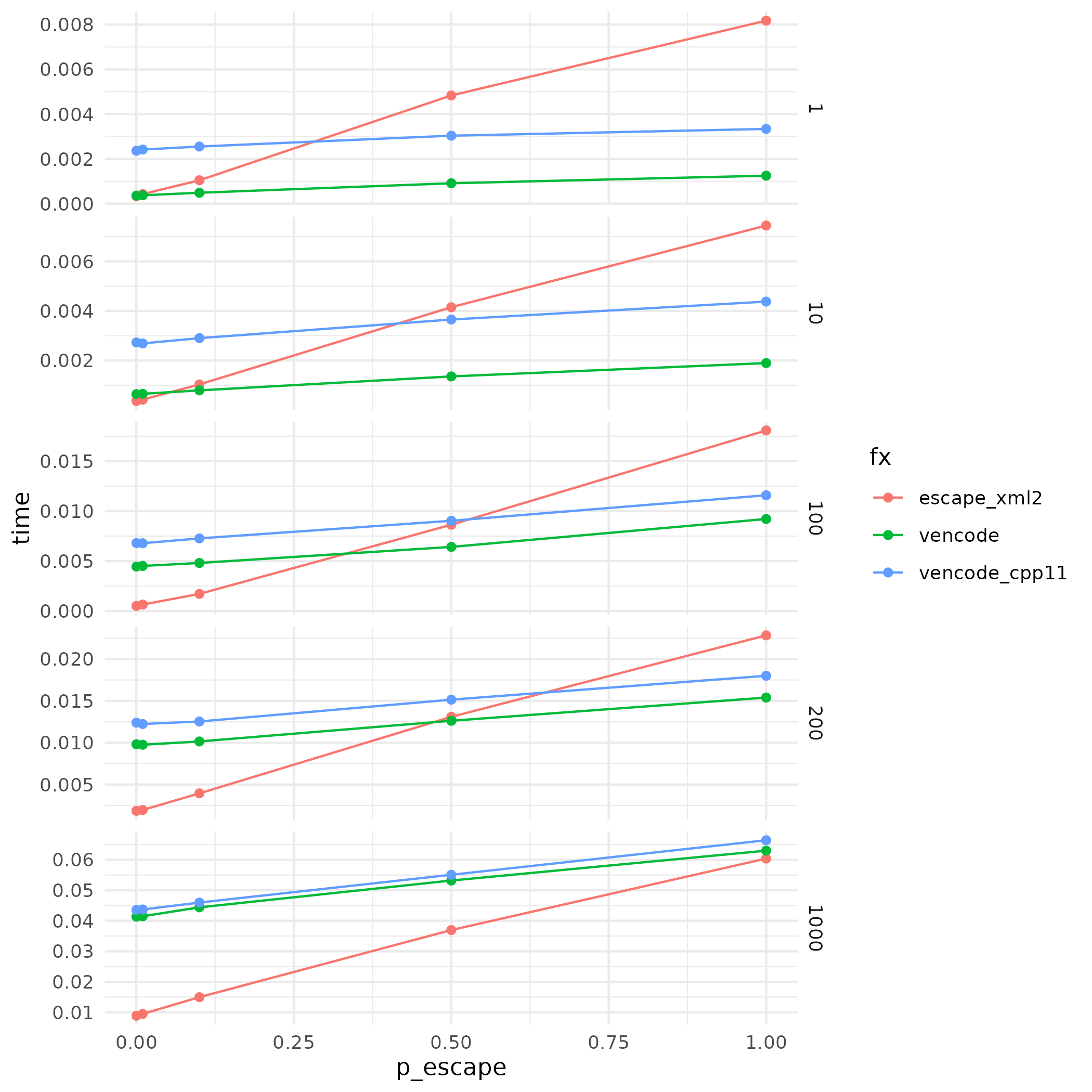
The performance profile suggests that cpp11 is consistently slower than Rcpp. But I must admit that my cpp11 implementation might not do justice to cpp11, although cpp11 and Rcpp implementations are line-by-line convertible. Probably not the most optimized way to do things in cpp11.
But how about going further? Well, next time. Also, the last time.