Werden wir Helden für einen Tag

Week 8: Super simple bayesian statistical inference with R

Posted on Feb 8, 2019 by Chung-hong Chan

firststep

The fact is, I am quite busy recently. But I don’t want to break the streak. So how about I write a quick one.

I have looked into bayesian statistics for few times in this blog. And I think most of you might know that the traditional frequentist statistical inference, for example, the P-value, is actually relying on P(X|H). Therefore, it is the conditional probability of having the data(X) as such or more extreme, when the null hypothesis(H) is true. Therefore, it is not correct to say thing like: because our p-value is very small, so our theory is true. The reason for this statement is wrong, is that p-value says nothing about how correct is your theory. It is all about the probability of observing such data, when the null is true.

Instead, what we usually want, is P(H|X), i.e. what is the probability of our hypothesis to be true, when we have the data as such. Such probability can be inferred by bayesian statistics.

A classical example in statistics is about flipping coin. For example, we flipped a coin for 20 times and observed 15 tails. Is this coin biased?

The traditional way of doing this, is to use the binomial test to calculate p-value. e.g.

binom.test(15, 20, p = 0.5, alternative = 'two.sided')
## 95%CI
## 0.5089541 0.9134285

By doing that we got a P-value of 0.0414. Using the traditional alpha < 0.05 criteria, we reject the null hypothesis. A correct conclusion from this binomial test is: when the null hypothesis is true, we have a probability of 0.0414 to have 15 tails or a more extreme version of the observation. Once again, it is P(X|H).

How about the P(H|X)? Well, it is actually not that difficult to compute that using R. To do bayesian statistics, we need three elements: prior, generative model and data.

Data is easy. Our “15 tails out of 20” is our data. Priors quantify our belief about the situation. For example, we don’t know exactly the probability of generating tails of our coin (P_t). It is equally likely to be from 0 to 1. The generative model is difficult to explain in word. I think it is easier for me to just do a simulation.

require(tidyverse)
n_samples <- 100000
prior_proportion_tails <- runif(n_samples, min = 0, max = 1)
n_tails <- rbinom(n = n_samples, size = 20, prob = prior_proportion_tails)
prior <- tibble(proportion_tails = prior_proportion_tails, n_tails)
posterior <- prior %>% filter(n_tails == 15)

par(mfrow = c(1,2))
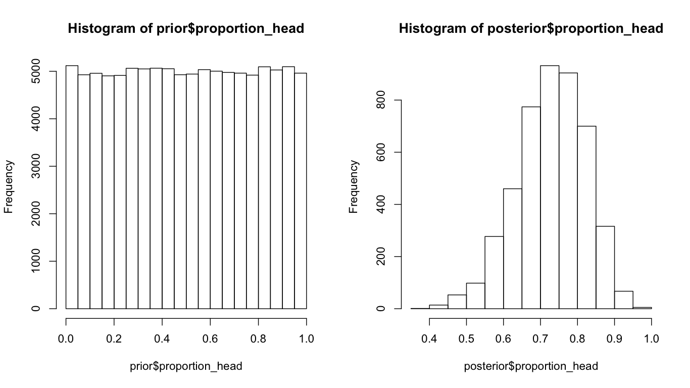
hist(prior$proportion_tails)
hist(posterior$proportion_tails)

quantile(posterior$proportion_tails, c(0.025, 0.975))

What we are trying to do here, is to simulate the possible outcomes (no of tails) with our prior belief (the P_t can be 0 to 1). With our data, select the outcomes from the prior fit our data. And then we study the posterior probability distribution of P_t. As we can see, the distribution of P_t shifts from a uniform distribution to a (log)normal distribution with the mean around 0.75. The beauty of bayesian statistics is that, we can say something like: given our data, it is 95% chance that P_t is from 0.53 to 0.89. Rather than saying, as in the (tedious) interpretation of confident interval: Upon replication of this experiment for many times and calculate the 95% CI for each replication, 95% of the time the true P_t is in those CIs. That is the difference between P(H|X) and P(X|H).

It is actually possible to do the bayesian inference more elegantly with out that large amount of simulated values.

prior_proportion_tails <- seq(0, 1, by = 0.01)
n_tails <- seq(0, 20, by = 1)
pars <- expand.grid(proportion_tails = prior_proportion_tails,
                    n_tails = n_tails) %>% as_tibble
pars$prior <- dunif(pars$proportion_tails, min = 0, max = 1)
pars$likelihood <- dbinom(pars$n_tails, 
                          size = 20, prob = pars$proportion_tails)
pars$probability <- pars$likelihood * pars$prior
pars$probability <- pars$probability / sum(pars$probability)
pars %>% filter(n_tails == 15) %>% mutate(probability = probability / sum(probability)) -> posterior
plot(y = posterior$probability, x = posterior$proportion_tails, type = 'l')

R is great as a tool to build this kind of bayesian intuition.

8 down, 44 to go.